Green Bottles

These last few days, I have been working on a new render—a green glass study. No big surprise there, as I'm a big fan of glass, refractions, reflections, caustics, dispersion, and anything related to rendering glass. There's something that just makes it never grow old. I used a photo I found on Facebook as reference, something I've been doing a lot recently. I find that real pictures taken by regular folks sometimes are more inspiring than perfect, professionally groomed pictures.

Also, for those interested, I gave a different subtext to the whole composition. I renamed the bottles to 1714-2014, in honor of the recent political events in Catalonia. Catalans are trying to have a referendum on independence in 2014, which marks the 300th anniversary of Spain's invasion and occupation of Catalonia. My bottles are literally freedom-water bottles! Not a bad reason to drink to.

As a side note, my blog has experienced a great increase in visits. As a way of saying thanks, I am including a link to the blend file and custom textures created by me. For the HDR image I use for the background, I would suggest using any that can easily be found online. Cheers!

Green bottles. Rendered in Cycles, modeled in Blender.
Click to enlarge.

This is the reference photo.

Creating Embroidery in Blender

A few months ago I posted this render of mine as a kind of homage to Barça's best ever coach: Pep Guardiola.

As a result, I got some positive feedback and some requests that I make a tutorial on how to create the embroidery effect. I must admit that, from my perspective, it is an embarrassingly simple matter, but I can understand (and remember) the feeling of being completely lost when it comes to particle systems and trying to reproduce randomly behaving stuff in Blender. That's why I feel a tutorial is a good idea. I am including a starter file with textures created by me, links and attribution to all external textures. I recommend using the latest builds of Blender (2.64 or 2.65 if possible), because I am using n-gons—polygons that have more than 4 edges—which were not supported in earlier versions of the program.

-Starter file just with my own textures
-NarrowPath_3k.hdr image from HDRLabs
-Wicker0020_15 from CGTextures

Before we go ahead with the tutorial proper, I want to suggest a simple exercise that will improve your chances of understanding how we are going to build this object. To sum it up, the embroidery effect was created with particle systems—specifically hair particle systems.

Particle systems are a kind of special effect used in many 3D packages that control the emission or distribution of other objects (particles) in potentially random and organic ways. In Blender, particle systems are applied to objects, which emit the particles along their normals. In my example, I have the Barça coat of arms shape as several polygonal objects, each of which has hairs of differing color and orientation applied to it.

Let's do this simple exercise. Open up a new blender file. Do not delete the default cube (I bet I surprised some blenderhead here). Make sure your cursor is on the 3D View window. Add another cube by pressing Shift-A, and then a 1 and a 2 (figure 1). Do not worry if you can't see the second cube. It's there, and it's called Cube.001. Without touching the mouse, scale the new cube down to 10% by pressing S and then . and 1 (figure 2). Notice we are not using the mouse or the cursor at all. Welcome to the power of Blender.

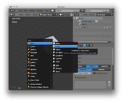
Figure 1. Press Shift-A and then 1 and 2 to create a new cube.

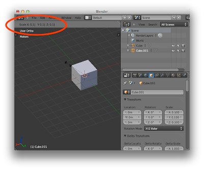
Figure 2. Press S, and then . and 1 to scale down to 10%.
Notice the info bar (upper left) reflects the scaling being applied.

Select the first cube by left-clicking on its name in the Outliner panel. Switch to the particles panel by clicking on the icon shown on figure 3. Click on the plus sign that shows up below to add a new particle system.

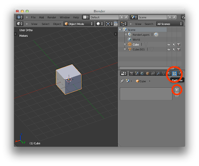
Figure 3. Switch to the Particles panel by clicking on the particle icon shown here.
Click on the plus sign to add a new particle system.

Notice that the newly created particle system is called by default ParticleSystem, and the settings used by this particle system are also called the same. In the drop down menu next to Type, select Hair (figure 4). You should see something like this:

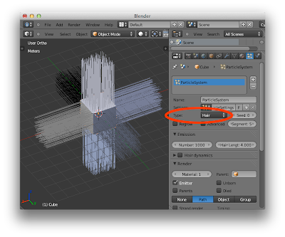
Figure 4. Select Hair as type in the drop down menu. The cube has hair now.

Scroll down the hair panel to find the Render sub-panel. Click on Object. In the Dupli Object (stands for duplicate object) field, type Cube.001 or click and select Cube.001. The original hairs get replaced by the tiny cubes. They are tiny because their size is, by default, 0.05, as specified in the Size field (figure 5).

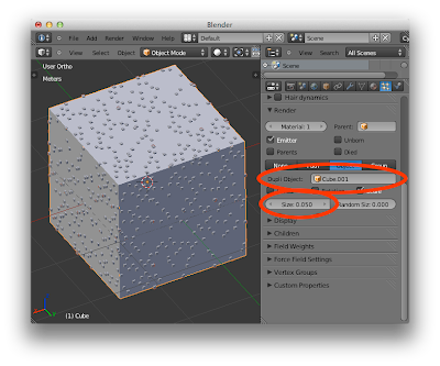
Figure 5. Notice that Cube.001 is what is being reproduced on the original cube, at a size
of 0.05 over the 10% reduced cube. I have zoomed in the scene so the tiny cubes can be seen.

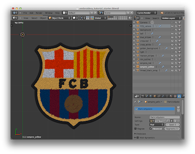
That's it for the introduction to particles. Let's build our Barça file now. Open the file embroidery_tutorial_starter.blend I provided in a link above.

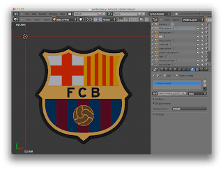
Figure 6. Starter file.

This file has all the objects and materials needed to create and render the scene. You might need to re-link the image textures that I am not including in the download. Since I am focusing mostly on using particle systems, I won't explain how to do this here. Some objects, like the light and the background are hidden from view, but they will render nevertheless. The individual embroidery stitches used for the different particle systems are all stored on layer 5 (see figure 7).

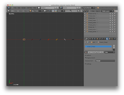
Figure 7. Layer number 5 contains the individual stitches, the hairs that will be used
to fill in the Barça coat of arms shapes with the embroidered effect.

Click on layer 1, and Shift-click layers 2, and 3 to activate them. Select the object named ball by clicking on it in the Outliner panel. Switch to the Particles panel if necessary. The object does not have any particle system applied to it yet. Click on the plus sign to add a new particle system. I already created the settings I use for all the different objects, and made sure they will be saved even of they are not actively being used in the file (by highlighting the F icon next to the particle settings name). Click on the ParticleSettings drop-down menu and select the Brown Thread settings (figure 8). There are many many settings that control how the emitted or hair objects behave in a particle system. Rather than bog you down with all these, just use the settings I have already created, and play with them once you feel comfortable enough.

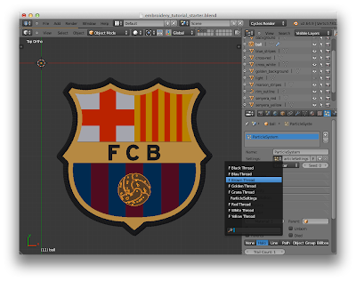
Figure 8. Select the Brown Thread settings to apply them to the ball object.

Keep selecting other objects in the scene and apply the pertinent particle system to each of them. Here is a list of objects with their corresponding particle setting:

-ball: Brown Thread
-blue stripes: Blau Thread
-cross_red: Red Thread
-cross_white: White Thread
-FCB_letters: Black Thread
-golden_background: Golden Thread
-maroon_stripes: Grana Thread
-senyera_red: Red Thread
-senyera_yellow: Yellow Thread

Notice that the stitches around the edge were created differently. They are using a path that controls the arrangement of an object around it. By now you should see something like this:

Figure 9. What things look like on the 3D View.

Just hit F12 now and let it render. Here is the result (figure 10), which took 3 minutes 34 seconds on my machine. I need a better Mac! You can fiddle around with the lighting, materials, or camera settings to give it a different look. Good luck and show me your results, and don't forget to press F3 to save the render!

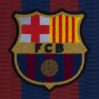
Figure 10. This is the basic render you'll get. My final render at the
top of the page had different lighting and some post-processing
applied to it.

Ear Reddening Render

This is my latest render. I've been getting back into go, and I like having go-related backgrounds on my computer. I usually search online for pictures or Japanese prints, and place them as wallpapers. One of these is the photo shown below, which apparently comes from this site.

Ear reddening game reference photo. 

The problem is that it is pretty low rez. So I decided to recreate it, using my existing goban scene, but modifying it a bit, and of course placing a bunch of additional stones on the board, up to the ear reddening move. Here is the result. Feel free to download it and use it as your desktop image.

I created the kanji letters (which read ear reddening move) in Illustrator.
I imported them as SVG into Blender, and placed them in a separate scene.
I combined both renders in the node compositor after that
—you can choose specific scene renders as separate inputs.

For those who don't know, the ear reddening move is a famous move in go lore. Played by Honinbo Shusaku against his rival Inoue Genan Inseki, it is the perfect move that managed to radically change the pace of an almost lost game for Shusaku (he fell into a joseki trap at the beginning of the game), and allowed him to turn the tables on his opponent. The move is called ear reddening because, according to legend, after the game one of the onlookers, not a go player himself, commented that he was sure Shusaku would end up winning the game because he saw Genan's ears get red upon seeing this move. My Cycles render did not take that long, so it wasn't very ear-reddening after all :)

About Strata Design 3D's Interface

Some of you might be wondering why I don't update this site as often as I used to. To that question, my only answer is that I've been looking for work (which, as they say, is a job in itself). Although I was looking in the graphic arts and prepress field, where I have some reasonable, real-world experience, I was lucky enough to land a job where, in addition to that, I'll actually have some possibility of using my 3D knowledge—and Blender. Most of the time I still pretty much battle with Illustrator files, PDF output, and plate generation. I like working with Illustrator, so that's really fine by me. However, as I said, I am also starting to do some 3D related work, mostly product visualization. Right now I am working on a product shot scene that takes full advantage of Blender particles and Cycles rendering capabilities.

Anyway, the company owns a copy of a 3D package I had never had the chance to use before: Strata Design 3D. I have started learning it, and so far my conclusion is that it probably has the best interface of any 3D package I've ever worked with (Blender, Cheetah3D, Maya, modo, Cinema4D, ZBrush, DAZStudio). Many keyboard shortcuts in Strata Design 3D are very similar to those associated with Illustrator or Photoshop.

For example, to move around the scene, you just press the space bar and drag (as in Illustrator/Photoshop), and to zoom in and out you add the Command or Command-Option keys to that (I work on a Mac after all), again like Illustrator/Photoshop. Another example is Option-drag to copy elements in the scene—finally a 3D program that gets it! The great thing is that there is, strictly speaking, no selection tool. Every tool (for example, move, rotate, scale) lets you select. Also, if you Option-drag an object with, say, the Rotate Tool selected, you'll rotate around the object's origin (or whatever origin you set) while duplicating. Blender's use of the Shift-D key combination to duplicate and immediately pressing one of the basic editing tools (G, S, R for grab, scale, rotate) is the only thing that can match Strata's speed while performing this simple task.

One other great user interface feature is the use of expandable side-tabs next to the options in some of the palettes—like the Image Texture palette (see figure 2). This arrangement manages to pack incredible amounts of easily accessible functions without cluttering the screen. Whoever designed Strata's user interface was paying attention.

Anyway, I still have a lot to learn about Strata, a deceivingly simple program that seems to have very powerful features. Right now I'm learning about material setup, lighting, global illumination, and efficient render settings. I'll try to keep you posted with my progress (not much to show yet).

Here are two screenshots of the program's UI. The first one is the minimalistic, context aware, and extremely useful Tool Palette. The second one is a screenshot of the Image Texture palette, perhaps the best organized material setup window I've seen in a 3D program. Great job!

Figure 1. Tool Palette

Figure 2. The Image Texture palette (or window?). Notice the side tab (Diffuse Amount) on he left,  that expands when you click on the double arrow below the eye on the far left of the highlighted Diffuse Amount context. Very efficient arrangement!

Using Takes in Cheetah3D

I've been wanting to write a simple tutorial on the basics of using Takes in Cheetah3D for a while. Finally I think I have it. Let me know if you find it useful! :)

What are takes? Takes are like scenes of a movie. Each take can store animation keys (recorded positions and parameters) that make it possible to have different scenes from one single set of 3D objects in the same file. Here is how takes are described in the Cheetah3D help files:

The take manager is a very powerful tool when it come to creating independent animation takes or clips. For example if you have a big architectural model and you want to create several independent camera fly throughs of a building. Another area where takes are very important is in the creation of animated characters for 3D games. These characters can perform various movements like running, jumping, kicking and so on. With the take manager you can record each of these animation into its own take.

In order to access takes, you need to switch to the Takes Manager, which is located by default in its own tab right next to the Object browser tag (figure 1).

Figure 1. The Takes panel—seen here
in its own tage by default.

You should notice a few things here. First, if you double-click on a take name, you can enter a different name for it. Second, you can change the take's length (measured in seconds) by double-clicking on the number next to the take name in the Length column, and entering a number (decimals allowed). Third, you can create more than one take per file. In order to do so, Control-click (or Right-click) on the panel, and choose New Take in the pop-up menu that appears (figure 2).

Figure 2. Right-click (or Control-click) on the Takes manager
to bring up a pop-up menu. Choose New Take to add more
takes to the file.

Some more pieces of information are necessary before you can start using the Takes manager comfortably:

1. Once you create a take, you can't change its stacking order in the Takes manager (new feature request here). If you need one take to appear before another within the Takes manager, plan accordingly.
2. Also, in order to delete a take, just  highlight it by clicking on it in the Takes manager and hit the Delete key.
3. In order to switch from one take to another, make sure to click on the checkmark-box to the left of the take name in the Takes manager. Just highlighting the name of a take does not activate it (figure 3).
4. When a take is active, all animation keys you record stay with that take. This can cause a bit of trouble if you key one parameter in one take but not in another. Objects that have been keyed in one take but not in another will transfer over their settings from the last active take. For example, if you record the Visible in renderer option for an object in a specific scene, but forget to record the same parameter for it (at whatever setting) in another take, when you switch to the un-keyed scene, the object will show up or not depending on the last active take. I hope this is not too confusing :)

Figure 3. Scene 1 is the active take. It is 6 seconds long.
Scene 2 is highlighted—if you press the Delete key,
you'll remove it from the file.

With all this information, we are ready for the mini-tutorial. Open a new Cheetah3D file, create a box, and save the file. You should have something like figure 4 (my window is super-small).

Figure 4. A new Cheetah3D file with a box.

Click on the Takes manager tab and create two takes like I describe on figure 2. Give them any name and length (in seconds) you like. One of the two takes will be the active take—the one with the checkmark on.

Figure 5. Create two takes. You can copy my settings here, but it's not that
important if you do not.

Select the box and enter -5 in the X Position field on the Properties panel (figure 6). You'll notice that the box moves to the left—that's OK.

Figure 6. Enter -5 in the X Position field in the Properties panel.
We are still on take Scene 1 in my file.

The next thing we need to do is to make sure we can see the whole timeline. By the way, if you can't see the timeline, click on the clock icon in the Toolbar (figure 7).

Figure 7. Click on this icon in the Toolbar to display the Timeline.

To show the whole timeline, grab the grey bar right next to the frame number indicator in the Timeline and drag it to the right until it spans the whole available width (figure 8).

Figure 8. Drag the dark grey bar all the way to the right to cover the whole
lighter bar. In my example, this shows the whole 6 seconds available for Scene 2.

Now, we're going to record some keys. Make sure the Box is selected and that the frame selector is set to 0, and click on the red button to the left of the Timeline to record the position of the Box. Actually, we are recording other things as well, like its rotation and scale, but the only thing that's going to change is its position (figure 9).

Figure 9. Make sure the frame selector is set to the 0 position.
Click on the red button to record the position of the box.

With the box still selected, move the frame selector to the last frame of the take (180 in my example). Enter 5 in the Position field in the Properties panel. Do not worry if the box disappears from view—it's still there. Click on the record button to record the box's postion on this frame. You can play the animation (press the green arrow) and see the box move! Notice that each frame that contains recorded keys displays a blue line over it on the Timeline (figure 10).

Figure 10. Notice the blue markers on the Timeline that indicate recorded keys.
In my example, on frame 111 this is the interpolated position for the box.

The next thing we need to do is switch to a different take. Go to the Takes panel and checkmark it. The scene seems to not have changed at all. The box will still be in the same position. That's because, when there are no recorded keys for parameters that do have them in other takes, the settings get transferred over from the last active scene. Notice, however, that the recorded keys have gone away. More the frame selector on the Timeline to frame 0 and move, rotate, scale the box as you see fit. Click on the Record button to record that position, scale, or rotation. Move the frame selector to the last frame and go crazy again with the scale, position, and rotation for the box. Hit the Record button again. Play the animation now. The nice surprise is that, if you go back to take Scene 1, the animation on that take is still there. No need to duplicate files, objects. All your animations with a specific sets of objects can reside in one same file! Neat eh?

Daffodils—Final Scene

Here is my (most likely) final render of the Daffodil scene. I decided to add an HDR to get more interesting reflections on the glass. I set its intensity to a fairly low amount, so that the overall feel would not be lost. I rendered it to just 1000 samples in Cycles, because I wanted to keep some of the graininess, which sometimes can add interest to an image. I applied a bit of color correction in Photoshop.  At some point in the future, I would like to make a digital painting version of it, since the initial inspiration has always been 17th century paintings with high contrast between shadows and lights.

Another render from a different angle, with a slightly different setup.

A Celebration of Pep

Pep Guardiola, Barça's coach for the last four years, just lead his team one last time to win the final of the Spanish King's Cup against Athletic Bilbao. Barça won the match 3-0 :) Actually, the highlight of the game might have been the deafening booing of the Spanish anthem by the Catalans and the Basques right before the game.

Guardiola is, without a doubt, the most successful Barça coach ever. Actually, he might be the most successful European coach ever. During these last four years, his team has won something like 16 out of 20 possible titles—I'm citing from memory, so forgive me if the figures are not exact. Before he became Barça's coach, I used to be pretty disenchanted with the team, which was mostly composed of foreign players who had nothing to do with Barcelona or Catalonia. He changed all that. He built a team from the ground up, capitalizing on local talent. Even Messi, the world-famous soccer player, grew up as a player in the Barça academy. That is something to be proud of.

Anyway, I created a little scene in recognition to all this. Visca el Barça!

Model created in Blender. Rendered in Cycles.
For the embroidery, I made use of Blender's particle hair system.

A fine procedural wood material for Cycles—Dissected

Just yesterday, I discovered this forum thread on Blenderartists, entitled A fine procedural wood material for Cycles, where the author, wesdves, shares an incredibly complex and good looking procedural material created with Cycles nodes. The .blend file is available for download on his first post. Just taking a look at the node setup for this material is mind-boggling (figure 2). The author has groups of nodes within other groups of nodes, all interconnected, mixing together, doing weird math, and in the end you get this great, realistic-looking result:

Figure 1. I created my own scene, appended (Shift-F1) the Wood material,
assigned it to a subdivided cube, and hit Render. This is the result.

Figure 2. This is what the node setup for the Wood material looks like. This is just the tip of the iceberg :)
Click on it to see a larger version.

I decided to render the file at different node locations to see how this thing was put together. Here are some of these renders, explained. I hope not only to learn a bit more about nodes in general, but also to share this knowledge so that others can come up with similar crazy stuff.

The first thing I did was connect each one of the two Mix nodes that come out of the color nodes at the bottom of the window (figure 2), one at a time, and do a render of that (figures 3 and 4). After all, that's where the color is coming from. Notice that the color distribution on each of these two Mix nodes is controlled by the same Wood.Rings node group, which I rendered too (figure 5). This Wood.Rings node in turn gets some kind of information from two other node groups (Wood Gnarl, Grain and Stain, and Wood.Planks), originating all from the Object output of a Texture Coordinate node. Notice also that, against what I think should be standard procedure, the author has connected yellow outputs to blue outputs along the way. This is probably OK here, although I have to admit that it hurts my eyes :) 

Figure 3. Result of rendering Mix 1.

Figure 4. Result of rendering Mix 2.

Figure 5. This is what you get when you connect the Wood.Rings
group into the Color input socket of the Glossy BSDF node and render it. 

Since a mix node puts these two outputs (figures 3 and 4) together through a third input (figure 5), I figured that's the same as having two images layered in Photoshop and mixing them through an alpha channel. So that's precisely what I did next. The result is shown on figures 6 and 7.

Figure 6. The final result of compositing figures 3 and 4 in Photoshop.
I think it's very similar to the final result in Cycles.

Figure 7. The Photoshop layers setup. I'm using an inverted version
of figure 5 as a layer mask to control the mix.

I continued doing some digging, connecting node outputs into the Glossy BSDF shader node, and here are some of the results I got.

Figure 8. This is what you get if you render the Object output
from the Texture Coordinate node. The colors depend on their
orientation in the local X Y Z space of the object. I think red is
for X, blue is for Z, and green for Y (not seen here,
only the yellow hints at it).

Figure 9. The result of rendering the Wood Gnarl, Grain and
Dirt node group.

Figure 10. The result of rendering the Wood Planks node group.
These last two are almost identical.

I'm going to try to dissect one of the node groups in this whole node setup. There is a lot of math that, frankly, I don't understand completely. Some of it seems superfluous and overly convoluted, but checking every step is a feat of back-engineering by itself, outside of the scope of this dissection exercise. I have a feeling that a simpler solution might have been possible in some areas—but I don't know fr sure right now. I'm going to focus on the Wood.Planks node group and try to have an intuitive sense for what it's doing. If you click on the Wood.Planks node and hit Tab, it expands, and it shows its contents (figures 11 and 12).

Figure 11. The collapsed Wood.Planks node group.

Figure 12. The Wood.Planks node group in all its splendor. Actually, not quite. notice more node groups inside of it :)

This Wood.Planks node group starts by separating the color components from the Object output in the Texture Coordinates node. If you render each of those three components you get the images shown on figures 13 to 15. Notice that they are greyscale, because each of the channels in an RGB image is defined in a scale from 0 to 1 (or 0 to 256, or whatever). An RGB color has three dimensions—a greyscale value has only one dimension.

Figure 13. Grayscale output for Red.

Figure 14. Grayscale output for Green.

Figure 15. Grayscale output for Blue.

 Each one of these separate channels goes through a conveyor-belt-like process that changes it a bit a time. The most important step is where they go through the node group named Wood.Modulator (figures 16 and 17) by its author. You can read about modulation is on Wikipedia's article about it. In the end, the images above get converted to what you see on figures 18 to 20.

Figure 16. The collapsed Wood.Modulator node group.

Figure 17. Expanded Wood.Modulator node group. Lots of math happening here. basically, the grayscale values are
subjected to division, rounding, subtraction, and multiplying with each other and with a starting value.

Figure 18. Red value after the modulation treatment.

Figure 19. Green value after the modulation treatment.

Figure 20. Blue value after the modulation treatment.

The Wood.Modulator node group has to outputs. So far, I looked at what the Frac output does. Here is what the Int output looks like:

Figure 21. Int output result.

I'm not going to continue with the remaining node groups. Some of them incorporate procedural textures modified with math—which gives the wood grain look. Also, you probably get the idea by now of how to begin to dissect a node setup and how to go about analyzing things. Someone on the forums mentioned that it would be great if there was some kind of system for adding comments to nodes. I think it would be a great thing to have—yet another tool for learning and sharing.